Plot a Disco Object

Visualize a causal graph stored within a Disco object. This function extends plot.Knowledge() by combining the causal graph from a caugi object with background knowledge.

Usage

# S3 method for class 'Disco'
plot(x, required_col = "blue", ...)

Arguments

x

A Disco object containing both the causal graph and the associated knowledge.

required_col

Character(1). Color for edges marked as "required". Default "blue".

...

Additional arguments passed to caugi::plot() and plot.Knowledge().

Value

Invisibly returns the underlying caugi object. The main effect is the plot.

Details

• Required edges are drawn in blue by default (required_col), can be changed.

• Forbidden edges are not drawn by.

• If tiered knowledge is provided, nodes are arranged according to their tiers.

• Other edge styling (line width, arrow size, etc.) can be supplied via edge_style. To override the color of a specific edge, specify it in edge_style$by_edge[[from]][[to]]$col.

This function combines the causal graph and the Knowledge object into a single plotting structure. If the knowledge contains tiers, nodes are laid out accordingly; otherwise, the default caugi layout is used. Edges marked as required are automatically colored (or can be overridden per edge using edge_style$by_edge).

See also

caugi::plot()

Examples

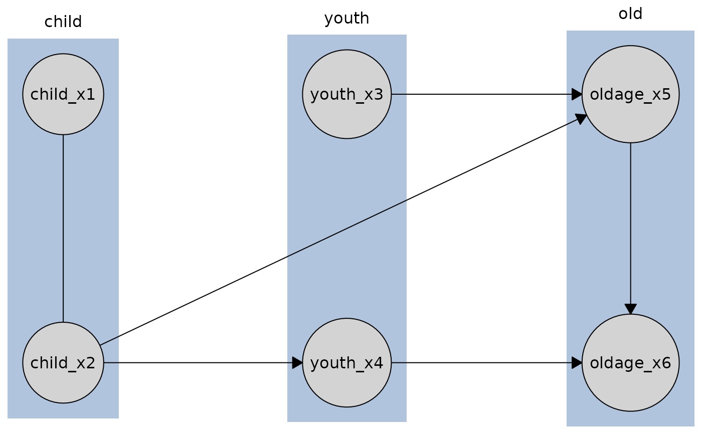
data(tpc_example)

# Define tiered knowledge
kn <- knowledge(
  tpc_example,
  tier(
    child ~ starts_with("child"),
    youth ~ starts_with("youth"),
    old ~ starts_with("old")
  )
)

# Fit a causal discovery model
cd_tges <- tges(engine = "causalDisco", score = "tbic")
disco_cd_tges <- disco(data = tpc_example, method = cd_tges, knowledge = kn)

# Plot with default column orientation
plot(disco_cd_tges)


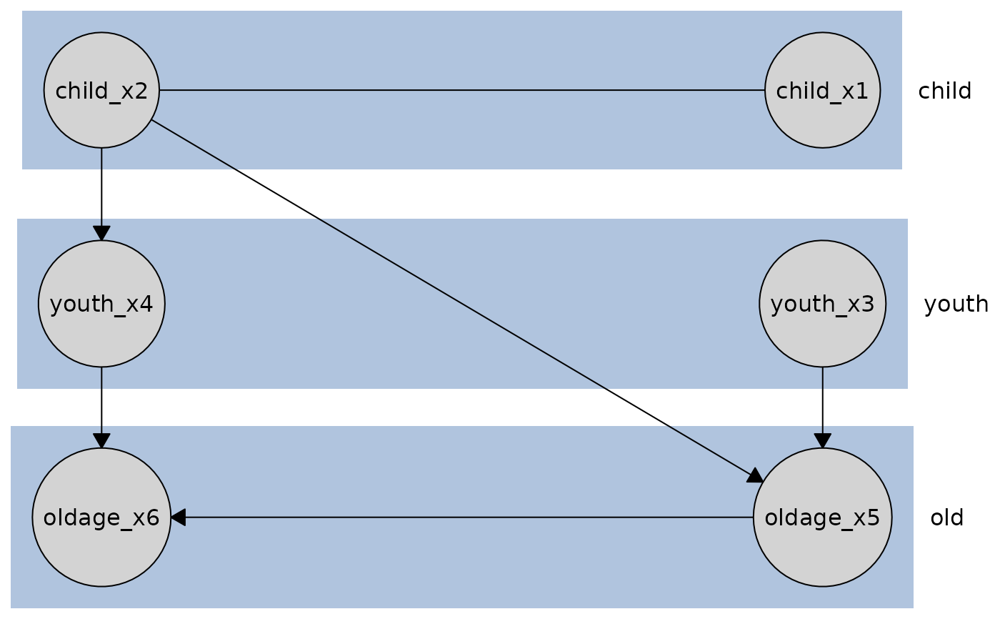
# Plot with row orientation
plot(disco_cd_tges, orientation = "rows")


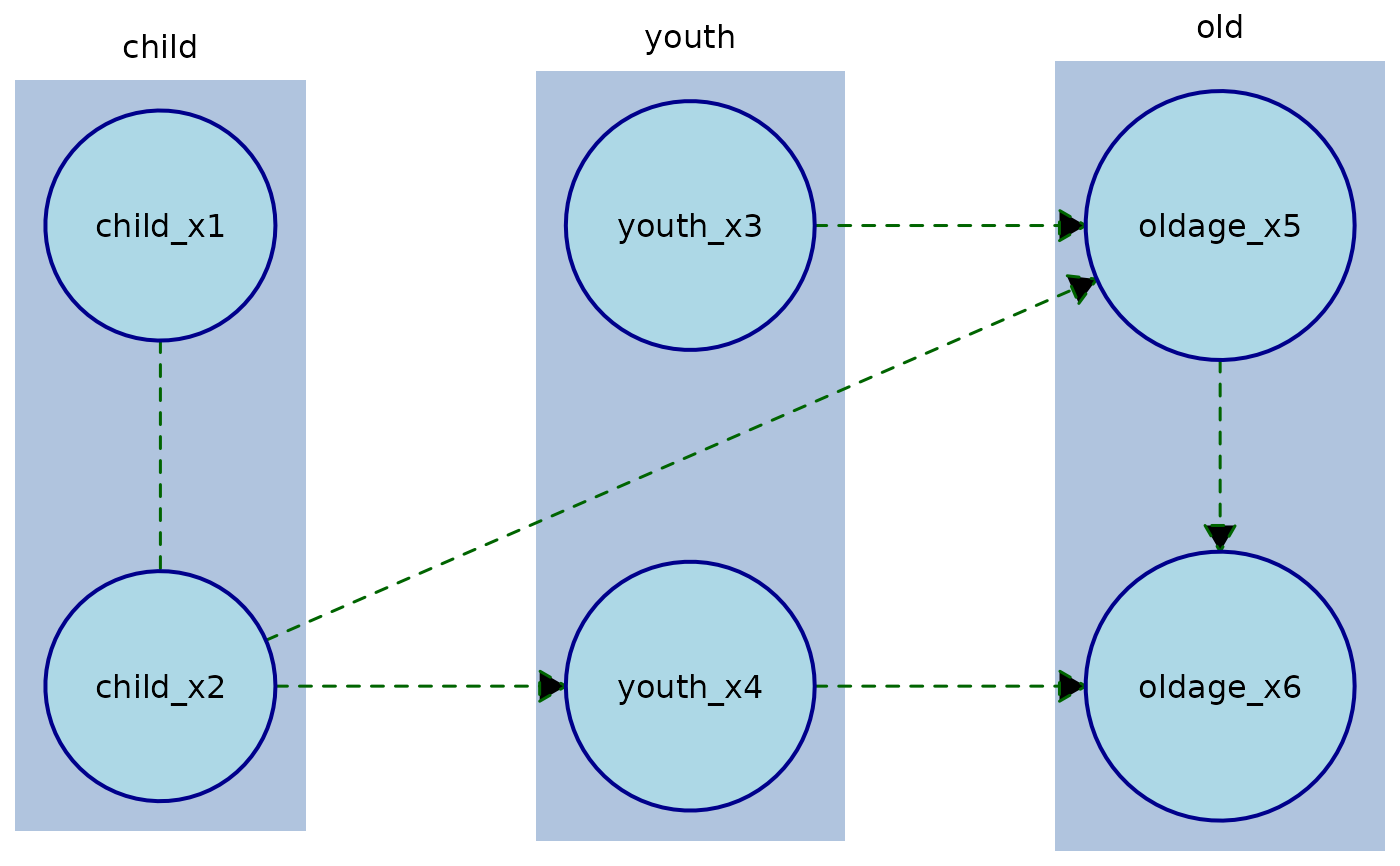
# Plot with custom node and edge styling
plot(
  disco_cd_tges,
  node_style = list(
    fill = "lightblue", # Fill color
    col = "darkblue", # Border color
    lwd = 2, # Border width
    padding = 4, # Text padding (mm)
    size = 1.2 # Size multiplier
  ),
  edge_style = list(
    lwd = 1.5, # Edge width
    arrow_size = 4, # Arrow size (mm)
    col = "darkgreen", # Edge color
    fill = "black", # Arrow fill color
    lty = "dashed" # Edge line type
  )
)


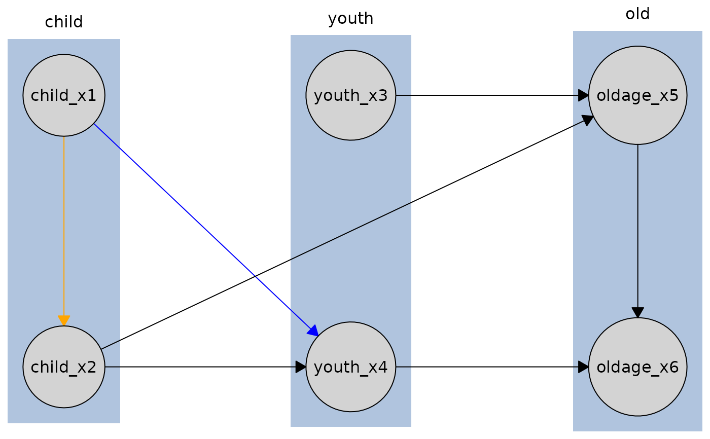
# To override a specific edge style which is required you need to target that individual node:
kn <- knowledge(
  tpc_example,
  tier(
    child ~ starts_with("child"),
    youth ~ starts_with("youth"),
    old ~ starts_with("old")
  ),
  child_x1 %-->% c(child_x2, youth_x4) # required edges
)
bnlearn_pc <- pc(engine = "bnlearn", test = "fisher_z")
disco_bnlearn_pc <- disco(data = tpc_example, method = bnlearn_pc, knowledge = kn)

# Edge from child_x1 to child_x2 will be orange, but edge from child_x1 to youth_x4
# will be required_col (blue) since we only override the child_x1 to child_x2 edge.
plot(
  disco_bnlearn_pc,
  edge_style = list(
    by_edge = list(
      child_x1 = list(
        child_x2 = list(col = "orange", fill = "orange")
      )
    )
  ),
  required_col = "blue"
)


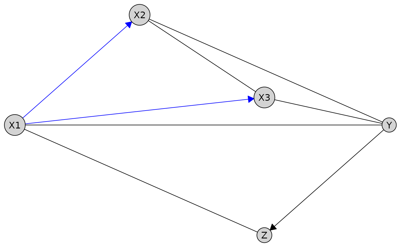
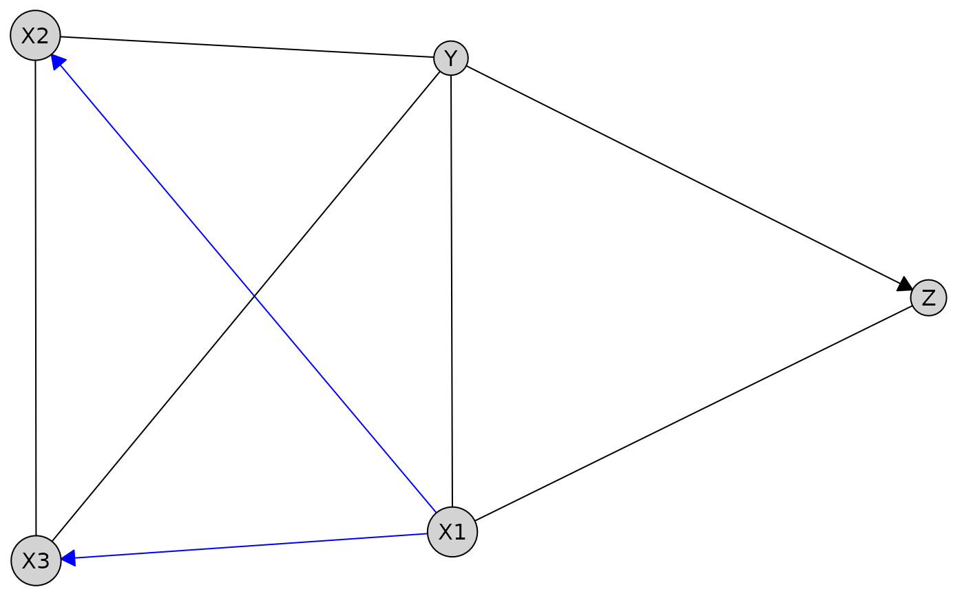
# Plot without tiers
data(num_data)
kn_untiered <- knowledge(
  num_data,
  X1 %-->% c(X2, X3),
  Z %!-->% Y
)

bnlearn_pc <- pc(engine = "bnlearn", test = "fisher_z")
res_untiered <- disco(data = num_data, method = bnlearn_pc, knowledge = kn_untiered)
plot(res_untiered)


# With a custom defined layout
custom_layout <- data.frame(
 name = c("X1", "X2", "X3", "Z", "Y"),
 x = c(0, 1, 2, 2, 3),
 y = c(0, 1, 0.25, -1, 0)
)
plot(res_untiered, layout = custom_layout)