
library(causalDisco)
#> causalDisco startup:
#>   Java heap size requested: 2 GB
#>   Tetrad version: 7.6.10
#>   Java successfully initialized with 2 GB.
#>   To change heap size, set options(java.heap.size = 'Ng') or Sys.setenv(JAVA_HEAP_SIZE = 'Ng') *before* loading.
#>   Restart R to apply changes.
This article demonstrates how to use the knowledge() function to incorporate prior knowledge into causal discovery algorithms. The supported knowledge types are introduced below, along with examples of creating Knowledge objects and using them with causal discovery methods.
At its core, all prior knowledge is represented as constraints on directed edges, specifying which edges are required or forbidden. Higher-level knowledge types provide more convenient ways to express common modeling assumptions, but ultimately translate into these edge constraints. All knowledge types can be freely combined: each call or operator adds constraints to the same Knowledge object. For example, requiring an edge from A to B and then requiring an edge from A to C produces a Knowledge object that requires both edges.
Required and forbidden knowledge
The most fundamental constraints are required and forbidden directed edges:
- Required edges specify that a directed edge must exist between two variables.
- Forbidden edges specify that a directed edge is not allowed between two variables.
These constraints are specified using the %-->% (required) and %!-->% (forbidden) operators. The exclamation mark (!) denotes negation of the edge, conceptually %!(-->)%, but we find this syntax too long.
Specifying required and forbidden edges
Suppose we want to require an edge from A to B, from A to C, and forbid an edge from B to C:
kn_1 <- knowledge(
  A %-->% B + C, # Require edges from A to B and A to C
  B %!-->% C # Forbid edge from B to C
)
This Knowledge object can be visualized:
plot(kn_1)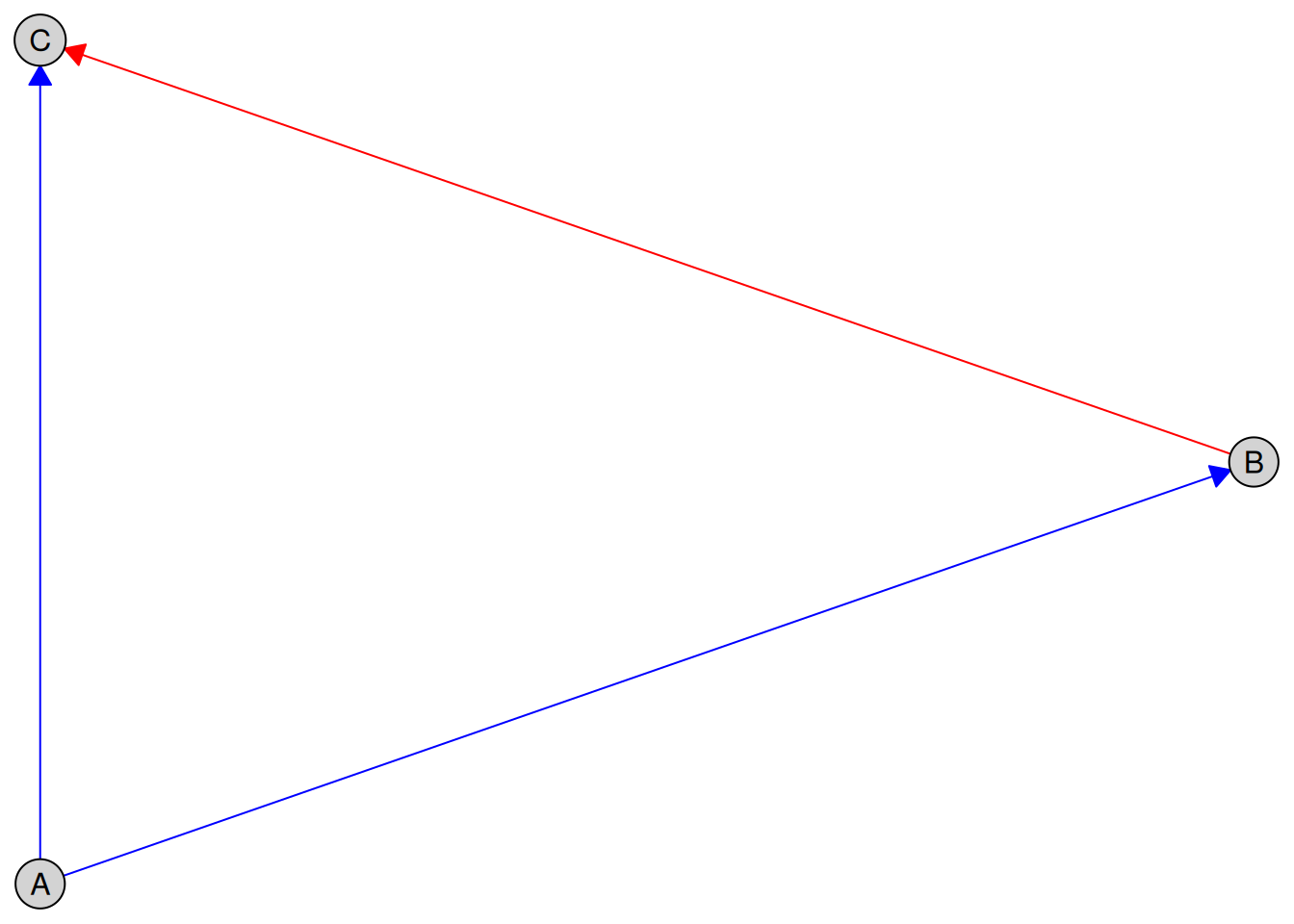
The blue edge represents the required edge from A to B, while the red edge represents the forbidden edge from B to C.
If one wishes to remove some edges (either required or forbidden) knowledge from existing Knowledge objects, the remove_edge() function can be used. For example, to remove the required edge from A to B:
kn_1_removed <- remove_edge(kn_1, from = A, to = B)
plot(kn_1_removed)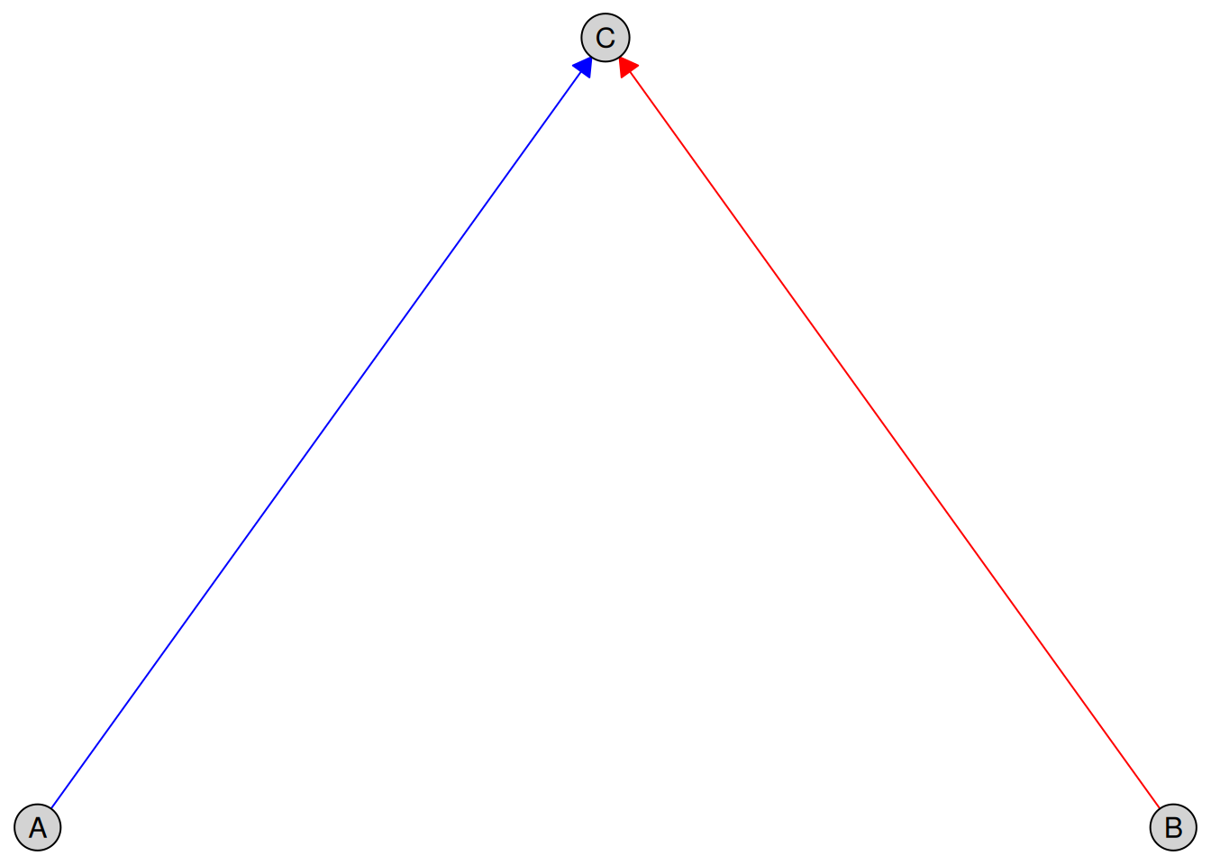
Specifying required and forbidden edges in a dataset
We will use the tpc_example dataset available in the package for the following examples. The dataset contains 6 variables, as shown below:
data(tpc_example)
head(tpc_example)
#>   child_x2   child_x1    youth_x4 youth_x3  oldage_x6  oldage_x5
#> 1        0 -0.7104066 -0.07355602        1  6.4984994  3.0740123
#> 2        0  0.2568837 -1.16865142        1  0.3254685  1.9726530
#> 3        0 -0.2466919 -0.63474826        1  4.1298927  1.9666697
#> 4        1  1.6524574  0.97115845        0 -7.9064009 -4.5160676
#> 5        0 -0.9516186  0.67069597        0  1.7089134  0.7903853
#> 6        1  1.9549723 -0.65054654        0 -6.9758928 -3.2107342
When specifying knowledge, it is often more convenient to specify the dataset so that the variables are checked for existence and selected correctly. To do this, pass the dataset as the first argument to knowledge().
kn_2 <- knowledge(
  tpc_example,
  child_x1 %-->% youth_x3, # Require edge from child_x1 to youth_x3
  child_x2 %!-->% oldage_x5 # Forbid edge from child_x2 to oldage_x5
)
This Knowledge object can also be visualized (we manually adjust the layout for better appearance):
cg <- knowledge_to_caugi(kn_2)$caugi
layout <- caugi::caugi_layout_sugiyama(cg)
layout[6, 2] <- layout[4, 2]

plot(kn_2, layout = layout)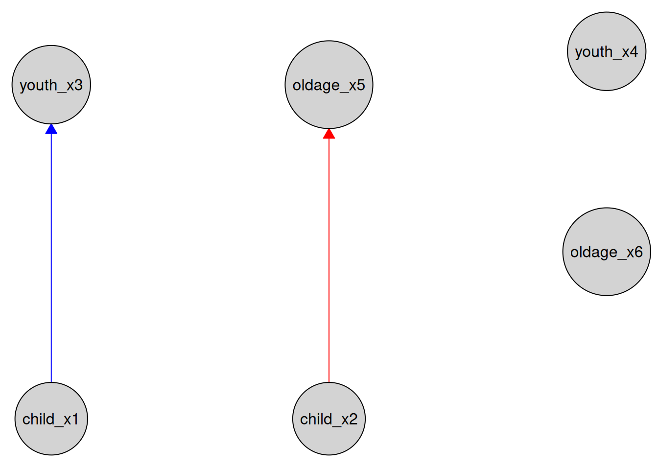
The plot then plots all variables in the dataset, with the required edges as blue edges and forbidden edges as red edges.
Using tidyselect helpers
To make specifying variables easier, you can use tidyselect helpers such as starts_with:
kn_3 <- knowledge(
  tpc_example,
  starts_with("child") %-->% starts_with("youth"),
  starts_with("oldage") %!-->% starts_with("youth")
)
This means, that all variables starting with “child” are required to have edges to all variables starting with “youth”, and no variables starting with “oldage” can have edges to any variables starting with “youth”. We can visualize this:
plot(kn_3)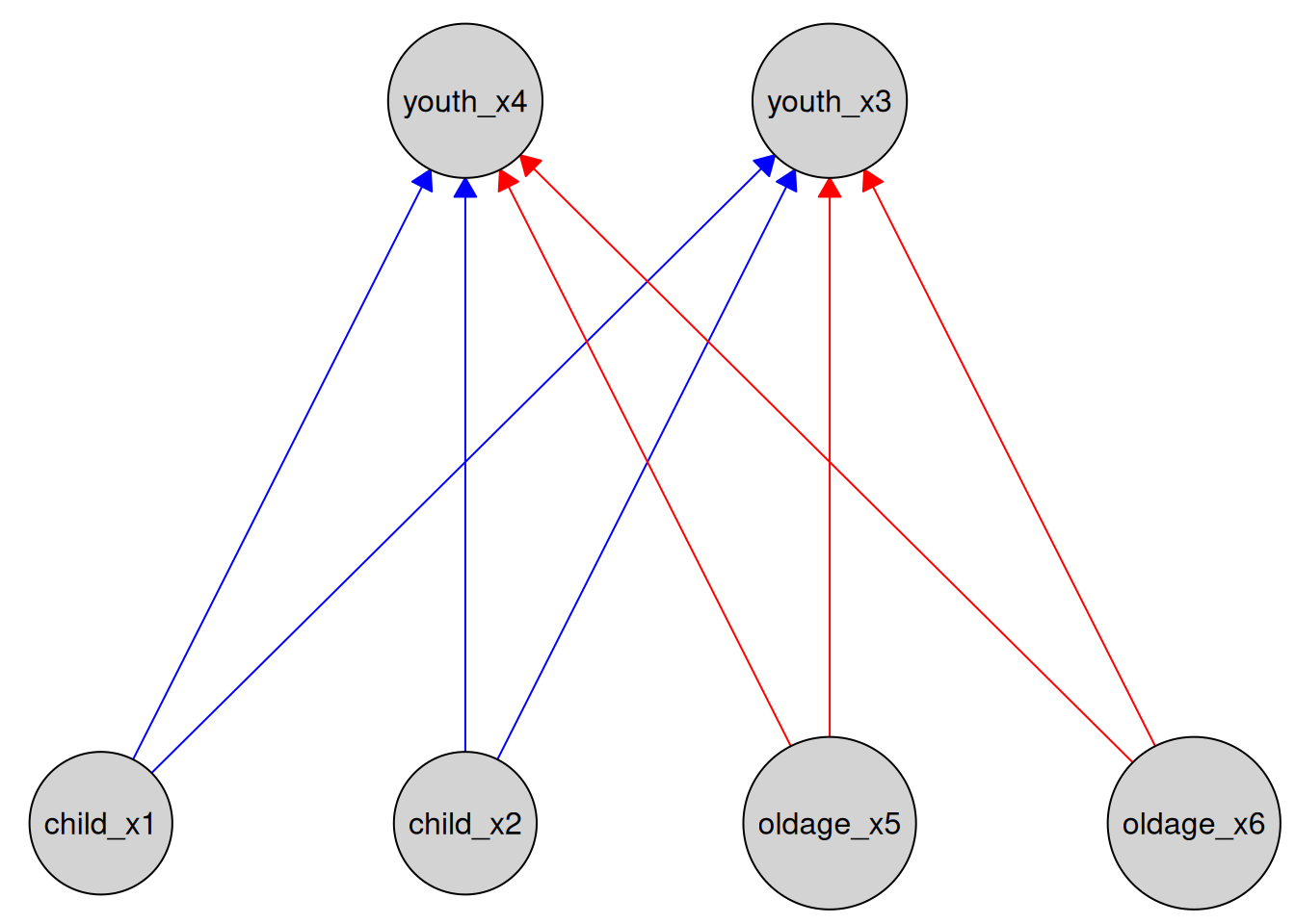
The tidyselect set operations ! (negation), & (intersection), and | (union) are also supported. For example, to forbid an edge from child_x1 to every variable that is not a “child” variable:
kn_4 <- knowledge(
  tpc_example,
  child_x1 %!-->% !starts_with("child")
)
For a list of all available tidyselect helpers we refer to the tidyselect reference documentation.
Tiered knowledge
Tiered knowledge provides a higher-level abstraction for expressing systematic ordering assumptions, such as temporal or logical precedence. Internally, tiered knowledge is translated into a collection of forbidden edges, but it is exposed separately because it provides a concise and structured way to express common ordering assumptions.
For example, consider a dataset with three groups of variables: child, youth, and old. We may wish to enforce that child variables precede youth variables, which in turn precede old variables. This can be expressed using tiered knowledge.
Tiered knowledge enforces that edges may only point from earlier tiers to later tiers. Edges within the same tier are unrestricted unless additional knowledge is supplied.
Creating a tiered Knowledge object
Suppose we observe variables over time: first the A’s, then the B’s, and finally the C’s. This ordering implies that causal direction cannot go backward in time (e.g., B’s cannot cause A’s). A tiered Knowledge object captures this temporal structure by specifying tiers and their associated variables. If numeric tiers are used, lower numbers indicate earlier tiers; otherwise, tiers are ordered by their appearance.
The following specifications encode the same tier structure:
kn <- knowledge(
  tier(
    1 ~ c(A1, A2),
    2 ~ c(B1, B2),
    3 ~ c(C1, C2)
  )
)

# Same object, since tiers are ordered numerically
kn_same <- knowledge(
  tier(
    1 ~ c(A1, A2),
    3 ~ c(C1, C2),
    2 ~ c(B1, B2)
  )
)

# Functionally equivalent, though not identical
kn_almost <- knowledge(
  tier(
    10 ~ c(A1, A2),
    30 ~ c(C1, C2),
    20 ~ c(B1, B2)
  )
)

# Again functionally equivalent
kn_also_almost <- knowledge(
  tier(
    A ~ c(A1, A2),
    B ~ c(B1, B2),
    C ~ c(C1, C2)
  )
)

# Has a letter, so tiers are ordered by appearance, thus functionally equivalent
kn_mixed <- knowledge(
  tier(
    3 ~ c(A1, A2),
    B ~ c(B1, B2),
    1 ~ c(C1, C2)
  )
)
We can visualize the tiers:
plot(kn)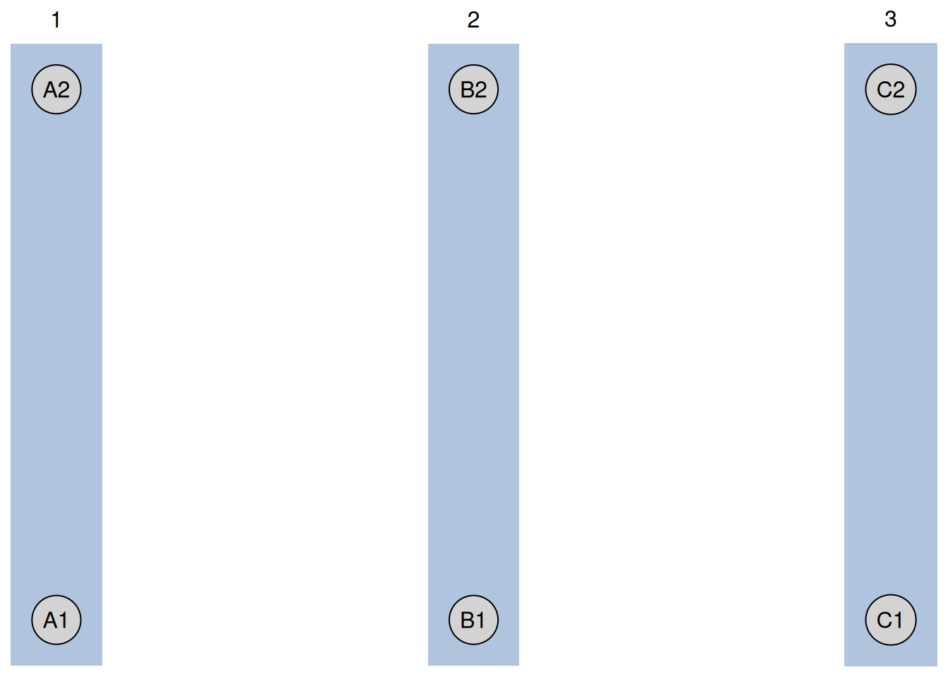
The plot then shows the tiers as layers, with the earliest tiers to the left and latest to the right.
We can convert the meaning of the tiered knowledge into explicit forbidden edges using convert_tiers_to_forbidden():
kn_converted <- convert_tiers_to_forbidden(kn)
print(kn_converted)
#> <Knowledge: 6 vars | 12 forbidden>
#>   vars: A1, A2, B1, B2, C1, C2
#>   forbidden:
#>     B1!-->A1 + A2
#>     B2!-->A1 + A2
#>     C1!-->A1 + A2 + B1 + B2
#>     C2!-->A1 + A2 + B1 + B2
plot(kn_converted)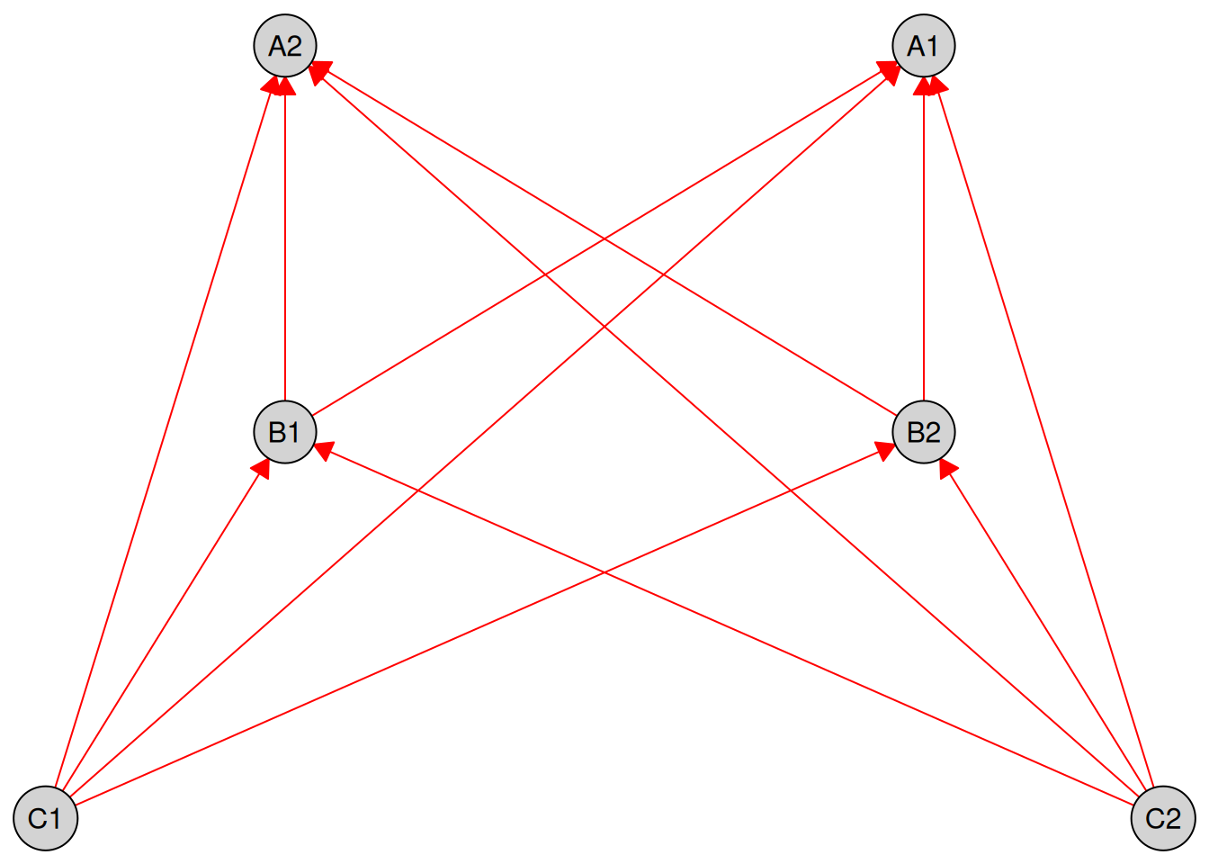
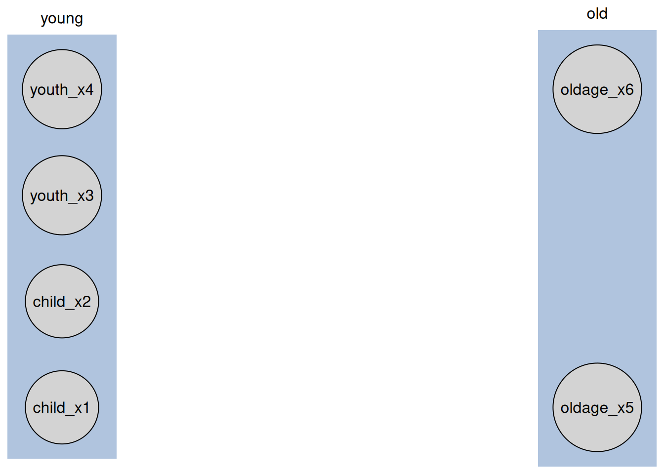
Tidyselect helpers such as starts_with can also be used to define tiers in a concise way, just as with required and forbidden edges. Different tidyselect helpers can be freely combined within a tier definition using +. For example, the following tiered Knowledge object defines two tiers, “young” and “old”, by combining tidyselect helpers on the variables in the tpc_example dataset:
Exogenous variables knowledge
Exogenous variables are those that have no incoming edges in the causal graph. That is, variables which are known causes but are not affected by other variables. Exogenous variables can be specified using the exogenous() function within knowledge().
Specifying exogenous variables
The most natural usage is to supply the dataset so that the variables are checked for existence and selected correctly:
kn_exo_1 <- knowledge(
  tpc_example,
  exogenous("child_x1")
)
Instead of exogenous(), you can also use the shorthand function exo(). This Knowledge object can be visualized:
plot(kn_exo_1)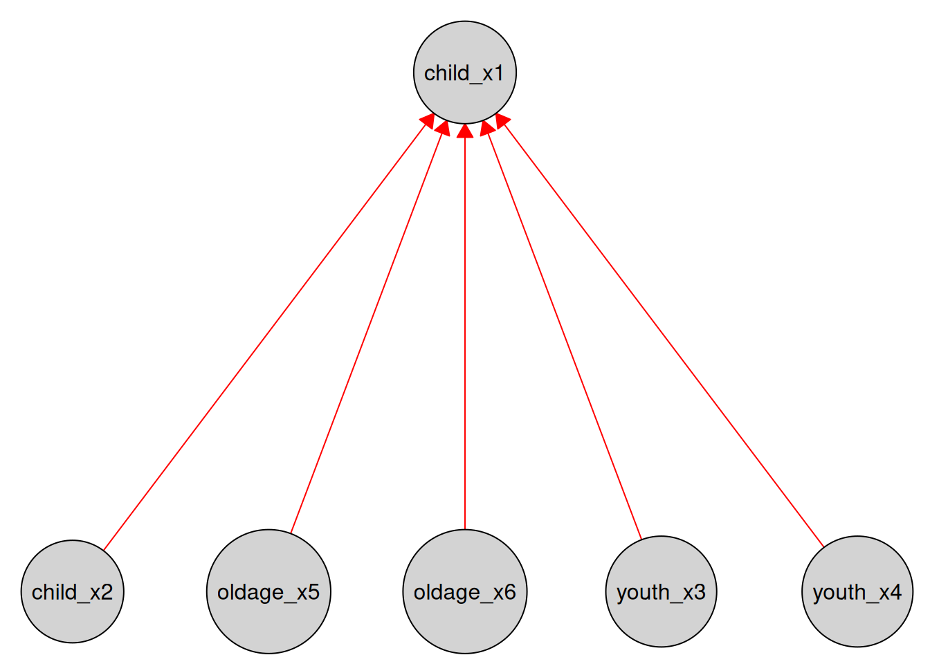
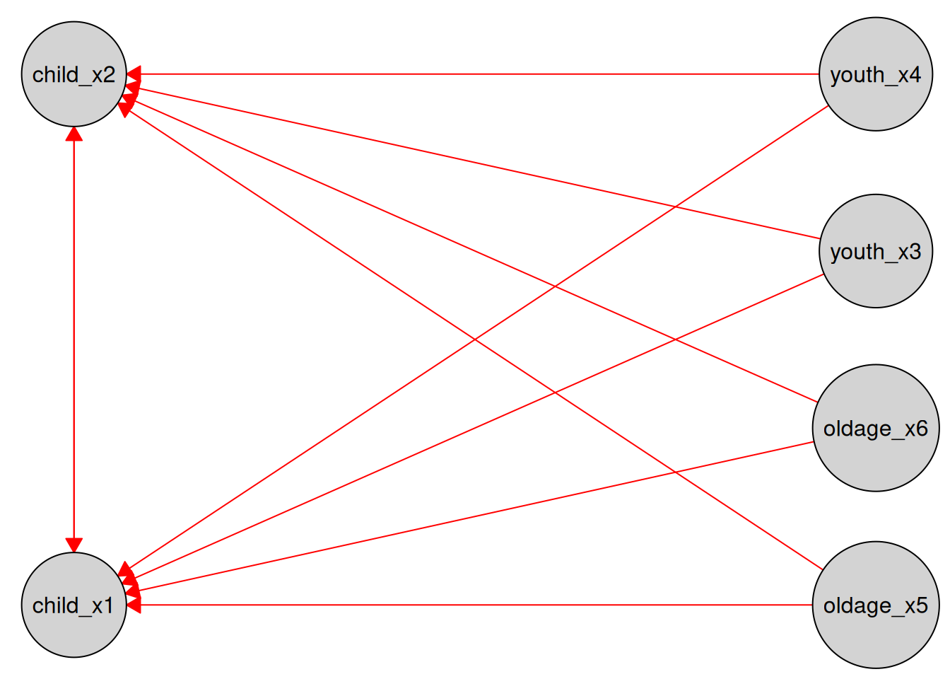
Below we add both child_x1 and child_x2 as exogenous variables using tidyselect helpers:
Combining different knowledge types
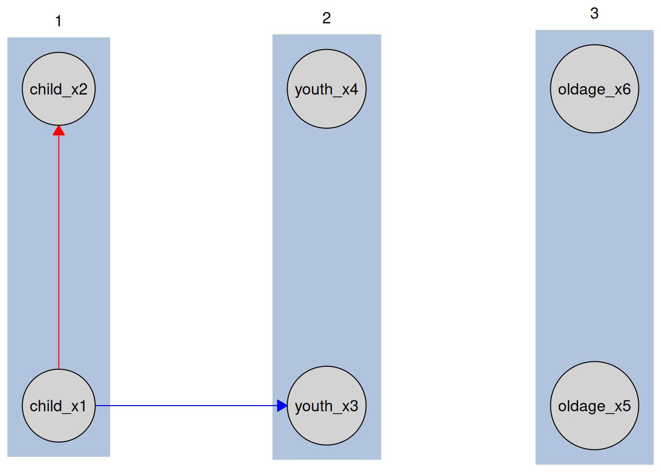
Different knowledge types can be freely combined in a single Knowledge object. For example, we can combine tiered knowledge with required and forbidden edges:
Using knowledge with causal discovery
Once prior knowledge has been specified, it can be supplied to causal discovery algorithms by passing the Knowledge object to the disco() function via the knowledge argument. For example, we can use the Temporal GES algorithm tges() with engine “causalDisco” and temporal BIC (“tbic”) score, while providing tiered knowledge:
The causal discovery algorithms will then learn the causal graph from the data given the constraints specified in the Knowledge object.
plot(disco_cd_tges)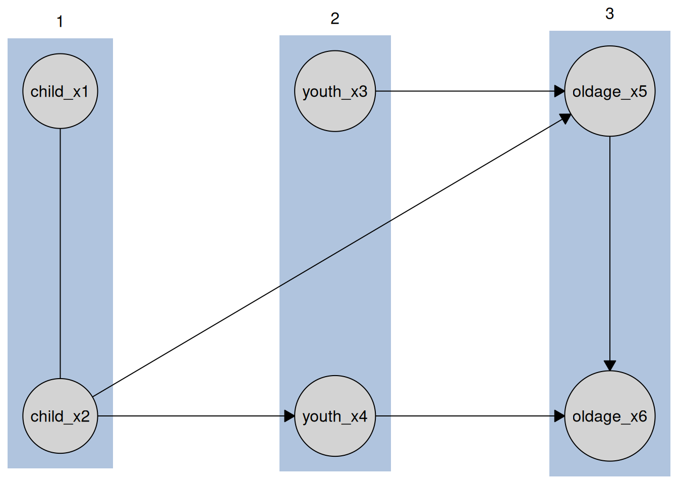
The black edges are those inferred from the data.
Engine specific information about knowledge
By engine we mean the underlying implementation of the causal discovery algorithm, i.e. the engine you specify to an algorithm such as pc(engine = "bnlearn") or tges(engine = "causalDisco").
Support for background-knowledge constraints differs across engines, as summarized in Table 1. The asterisks for causalDisco and pcalg indicate that only symmetric forbidden-edge constraints are supported, i.e. an edge must be forbidden in both directions. In addition, causalDisco automatically detects when a set of forbidden edges is equivalent to a tiered ordering and, in that case, treats it as tiered knowledge.
| Engine | Forbidden edges | Required edges | Tiered knowledge |
|---|---|---|---|
causalDisco |
✓* | ✓ | |
pcalg |
✓* | ||
bnlearn |
✓ | ✓ | ✓ |
Tetrad |
✓ | ✓ | ✓ |
bnlearn
When required knowledge is provided, bnlearn may emit a warning during structure learning. This occurs when the algorithm identifies a candidate v-structure (collider) from the data whose orientation conflicts with already oriented edges.
data(tpc_example)

kn <- knowledge(
  tpc_example,
  child_x1 %-->% youth_x3
)

bnlearn_pc <- pc(engine = "bnlearn", test = "fisher_z", alpha = 0.05)
output <- disco(data = tpc_example, method = bnlearn_pc, knowledge = kn)
#> Warning in vstruct.apply(arcs = arcs, vs = vs, nodes = nodes, debug = debug):
#> vstructure child_x2 -> oldage_x5 <- youth_x3 is not applicable, because one or
#> both arcs are oriented in the opposite direction.
The resulting causal graph will still respect the provided knowledge.
plot(output)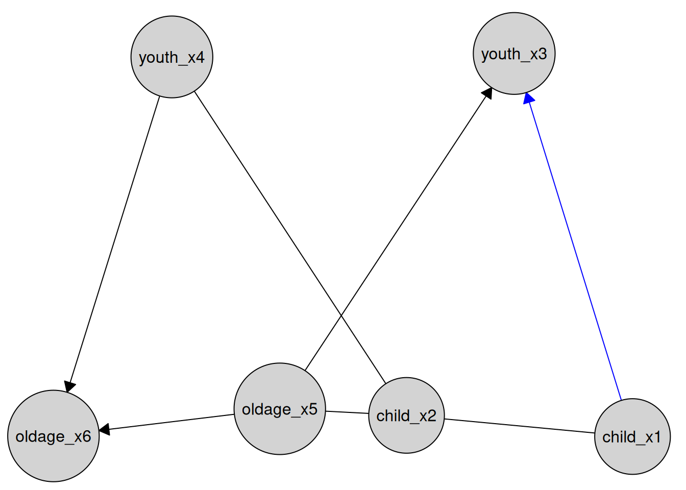
pcalg
Symmetric forbidden-edge constraints can be specified using %!-->% in both directions, as illustrated below:
causalDisco
Symmetric forbidden-edge constraints are also supported (as for pcalg above), in addition to directed forbidden edges that are equivalent to some tiered knowledge. For example, forbidding oldage from pointing to child is equivalent to placing child in the same tier as youth:
data(tpc_example)
kn <- knowledge(
  tpc_example,
  starts_with("oldage") %!-->% starts_with("child"),
  starts_with("oldage") %!-->% starts_with("youth"),
  tier(
    1 ~ starts_with("youth"),
    2 ~ starts_with("oldage")
  )
)
my_tpc <- tpc(test = "fisher_z", alpha = 0.05)
output <- disco(data = tpc_example, method = my_tpc, knowledge = kn)
#> The directed forbidden edges in `knowledge` place 2 untiered variable(s) in the temporal order; assigning them to tiers.
If the forbidden edges do not correspond to any tiered knowledge, an error is raised instead.