library(causalDisco)
#> causalDisco startup:
#>   Java heap size requested: 2 GB
#>   Tetrad version: 7.6.10
#>   Java successfully initialized with 2 GB.
#>   To change heap size, set options(java.heap.size = 'Ng') or Sys.setenv(JAVA_HEAP_SIZE = 'Ng') *before* loading.
#>   Restart R to apply changes.
This article provides a very brief introduction to causal discovery using simulated data. For a thorough introduction to causal discovery concepts, we recommend Glymour et al. (2019) Review of Causal Discovery Methods Based on Graphical Models or Zanga et al. (2022) A Survey on Causal Discovery: Theory and Practice.
The goal of causal discovery is to infer the causal relationships among a set of observed variables using observational data.
Example of causal discovery
Suppose we have this DAG:
cg <- caugi::caugi(
  Z %-->% X1,
  X3 %-->% X2,
  X1 %-->% Y,
  X2 %-->% Y
)
We define a layout which we will use for plotting the graphs in this article:
layout <- caugi::caugi_layout_sugiyama(cg)
plot(cg, layout = layout, main = "True DAG")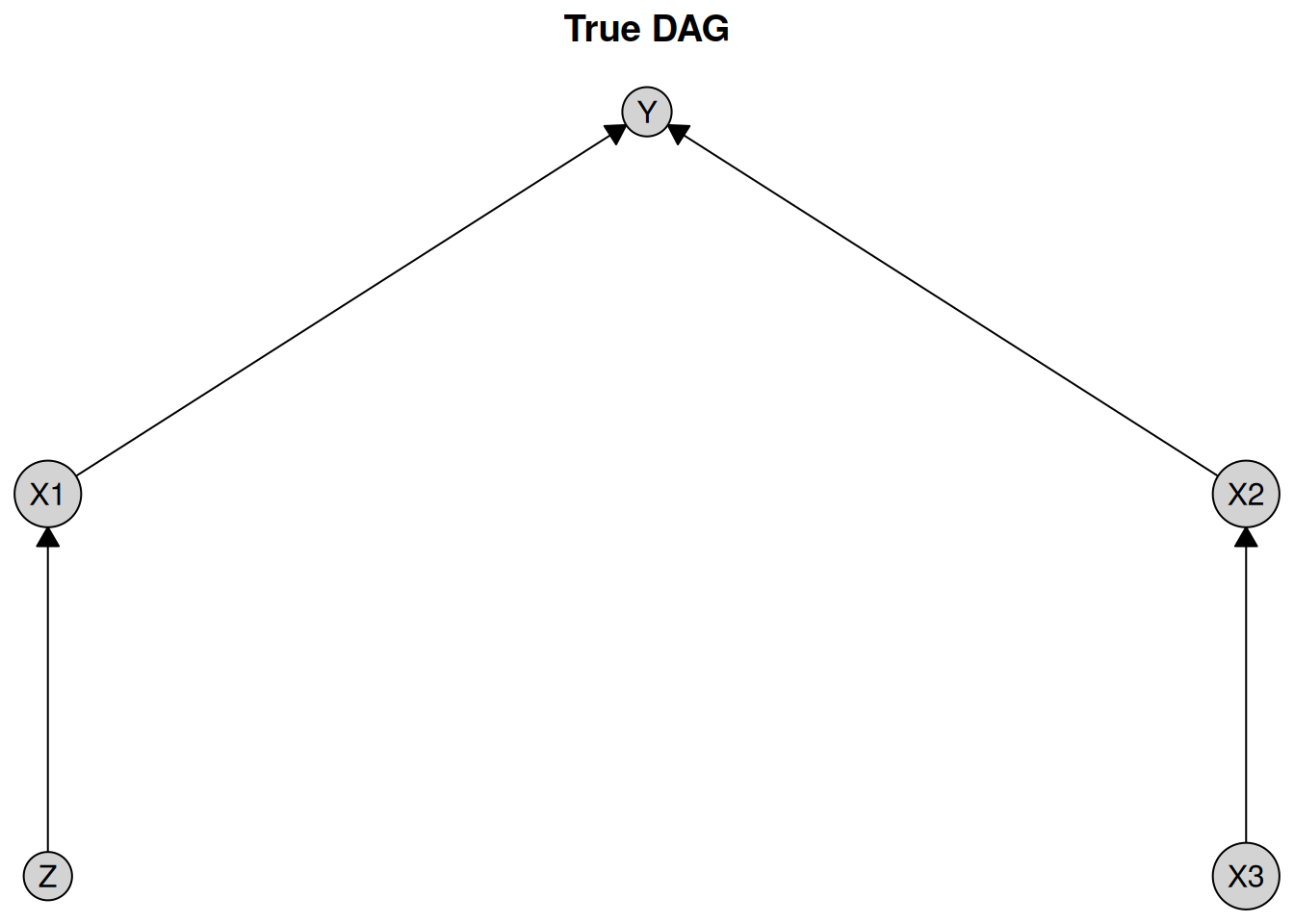
We can create data from a linear Gaussian model corresponding to the above DAG using generate_dag_data(). We generate 10,000 samples with a fixed random seed from the DAG above, where we let the edge coefficients be sampled with absolute values between 0.1 and 0.9 and assigned random signs, and where the standard deviation of the additive Gaussian noise at each node is sampled from a log-uniform distribution between 0.3 and 2.
data_linear <- generate_dag_data(
  cg,
  n = 10000,
  seed = 1405,
  coef_range = c(0.1, 0.9),
  error_sd = c(0.3, 2)
)
head(data_linear)
#> # A tibble: 6 × 5
#>        Z      X3     X1      X2       Y
#>    <dbl>   <dbl>  <dbl>   <dbl>   <dbl>
#> 1  0.632  0.297   0.773 -0.256  -0.730
#> 2 -1.67  -1.10   -1.20   1.10   -0.722
#> 3 -0.214  0.713   1.09   0.0264  0.261
#> 4 -1.61  -0.171  -1.21  -0.0346  0.0746
#> 5  1.57   0.0517  0.402 -0.874   1.40
#> 6 -1.08   0.178  -1.09   0.189   0.0591
The R code used to generate the data is stored as an attribute of the data frame:
attr(data_linear, "generating_model")
#> $dgp
#> $dgp$X3
#> rnorm(n, sd = 0.95)
#>
#> $dgp$X2
#> X3 * 0.159 + rnorm(n, sd = 0.507)
#>
#> $dgp$Z
#> rnorm(n, sd = 1.794)
#>
#> $dgp$X1
#> Z * 0.3 + rnorm(n, sd = 1.634)
#>
#> $dgp$Y
#> X1 * 0.61 + X2 * 0.31 + rnorm(n, sd = 1.216)
The goal is now to recover the causal structure from the data alone.
We will use the PC algorithm to learn the causal structure. One of its key assumptions is causal sufficiency, meaning that there are no unobserved confounders. We can use the PC algorithm from any of the “tetrad”, “pcalg”, or “bnlearn” engines to learn the structure from the data. The motivation for having multiple engines is that they may implement different algorithms, tests, or scoring methods, or the same algorithm may be implemented differently across engines.
Below, we set up the PC algorithm using Fisher’s Z test, a significance level of 0.05, and pcalg as the engine. To do so, we first define the PC method using the pc() function, and then pass it to the disco() function along with the data.
We can visualize the results using the plot() function, where we explicitly provide the layout defined above so graphs are easier to compare.
plot(pc_result_pcalg, layout = layout, main = "PC (pcalg)")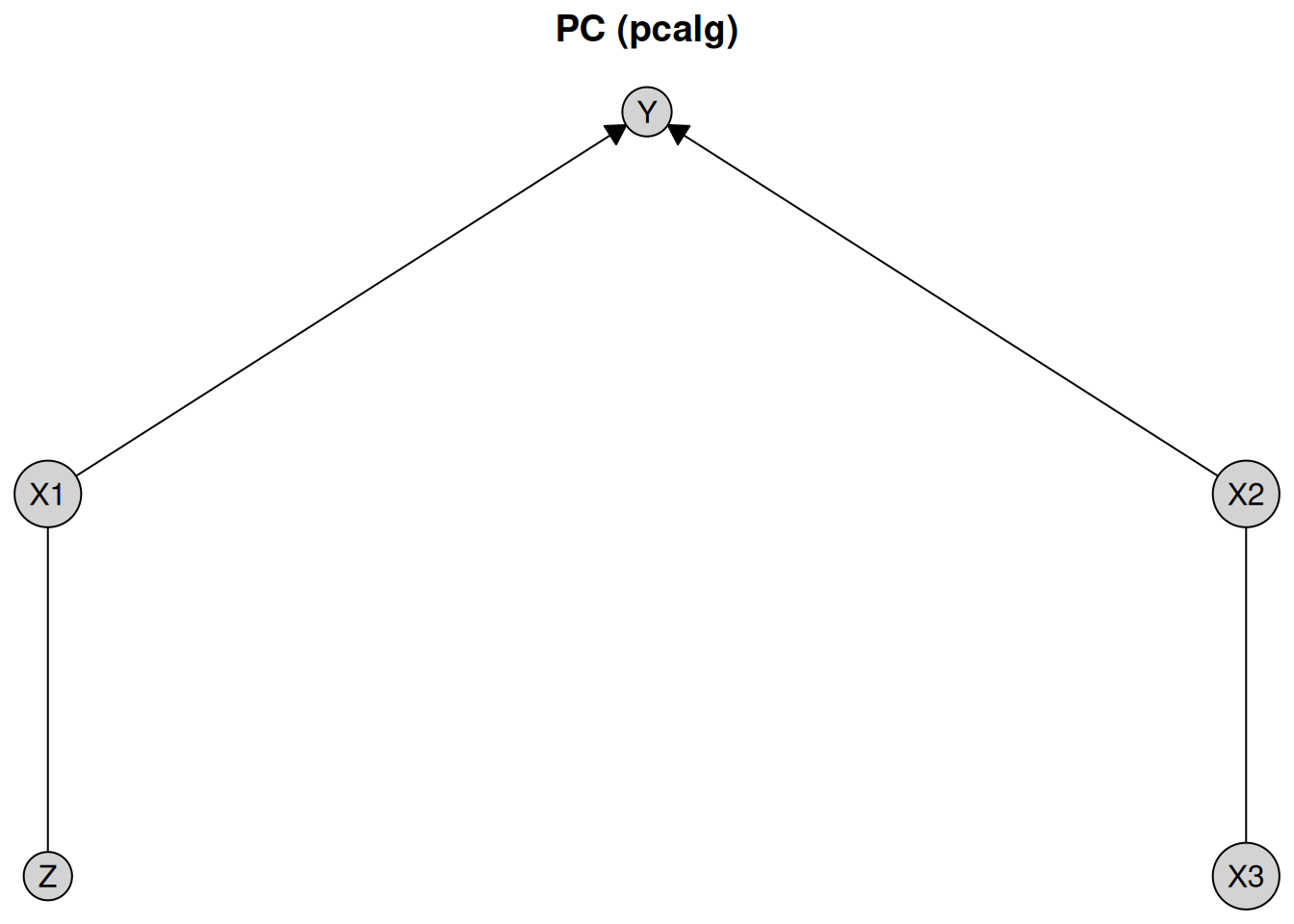
The PC algorithm recovers the correct causal structure up to Markov equivalence, represented as a CPDAG. A CPDAG represents the equivalence class of DAGs that encode the same conditional independencies.
The first notable feature of this plot is that some edges are directed, while others are undirected. For example, the edge from X1 to Y is directed, indicating a causal effect of X1 on Y, but not in the reverse direction. In contrast, the edge between X2 and X3 is undirected, indicating that the data alone do not provide sufficient information to determine the causal direction. Both orientations X2 %-->% X3 and X3 %-->% X2 are compatible with the observed conditional independencies.
We demonstrate the non-identifiability of the causal direction between X2 and X3 by reversing the direction of this edge in the data-generating process above and applying the PC algorithm to the resulting data set.
cg_reverse <- caugi::caugi(
  Z %-->% X1,
  X2 %-->% X3,
  X1 %-->% Y,
  X2 %-->% Y
)

data_linear_reverse <- generate_dag_data(
  cg_reverse,
  n = 10000,
  seed = 1405,
  coef_range = c(0.1, 0.9),
  error_sd = c(0.3, 2)
)

pc_result_reverse <- disco(data = data_linear_reverse, method = pc_pcalg)
plot(pc_result_reverse, layout = layout, main = "PC (pcalg) reversed")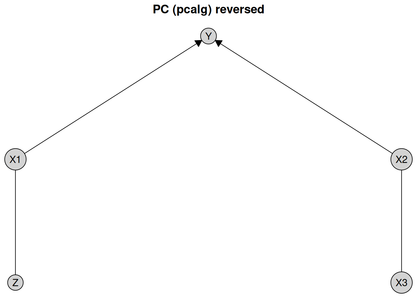
We learn the same causal structure as before, demonstrating that the direction of influence between X2 and X3 cannot be determined from the data alone.
Unobserved confounding
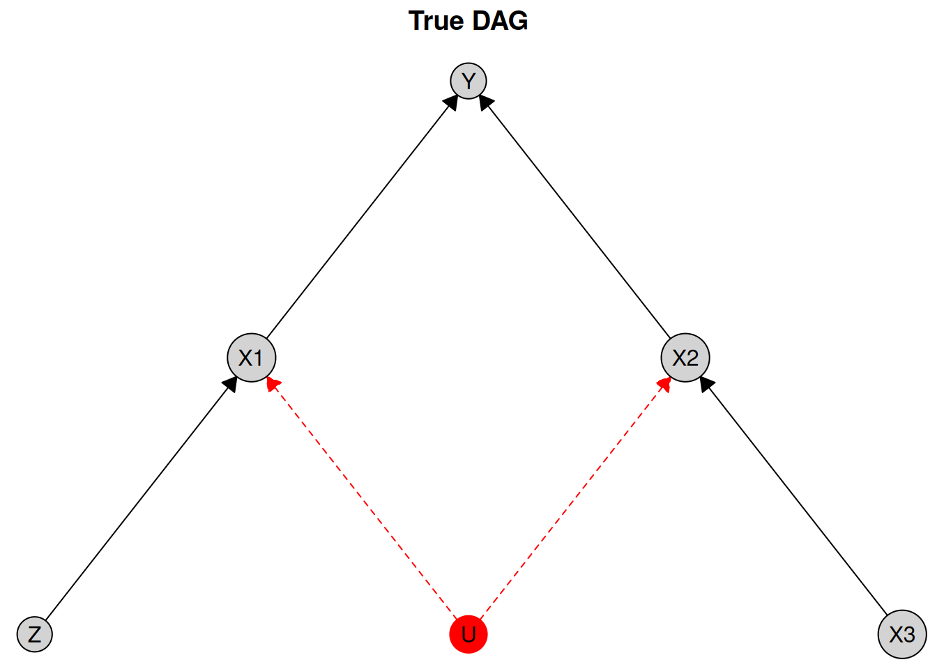
In practice, unobserved confounding may be present, violating one of the assumptions of the PC algorithm. Suppose we have the following DAG with an unobserved confounder U between X1 and X2:
cg_unobserved <- caugi::caugi(
  Z %-->% X1,
  X3 %-->% X2,
  X1 %-->% Y,
  X2 %-->% Y,
  U %-->% X1 + X2
)
We can visualize this DAG, marking the unobserved variable U in red and using dashed edges to indicate that it is unobserved:
plot(
  cg_unobserved,
  edge_style = list(
    by_edge = list(
      U = list(col = "red", fill = "red", lty = "dashed")
    )
  ),
  node_style = list(
    by_node = list(
      U = list(col = "red", fill = "red")
    )
  ),
  main = "True DAG"
)
We can generate data from this DAG using generate_dag_data(), and then afterwards remove the unobserved variable U from the data frame:
data_unobserved <- generate_dag_data(
  cg_unobserved,
  n = 10000,
  seed = 1405,
  coef_range = c(0.1, 0.9),
  error_sd = c(0.3, 2)
)
data_unobserved <- data_unobserved[, names(data_unobserved) != "U"]
head(data_unobserved)
#> # A tibble: 6 × 5
#>         Z      X3     X1     X2       Y
#>     <dbl>   <dbl>  <dbl>  <dbl>   <dbl>
#> 1  0.608   1.42   -1.31  -1.69   1.99
#> 2 -0.716  -0.357  -0.490 -0.561  0.955
#> 3  1.22    1.49   -0.124 -1.48   1.52
#> 4 -0.752  -0.188   0.877  1.35  -1.39
#> 5 -0.0863  0.0156  1.54  -0.926 -0.0833
#> 6 -0.799  -0.929   0.802  0.253 -0.939
We can then apply the PC algorithm as before:
pc_pcalg_unobserved <- pc(engine = "pcalg", test = "fisher_z", alpha = 0.05)
pc_result_unobserved <- disco(
  data = data_unobserved,
  method = pc_pcalg_unobserved
)
plot(pc_result_unobserved, layout = layout, main = "PC (pcalg)")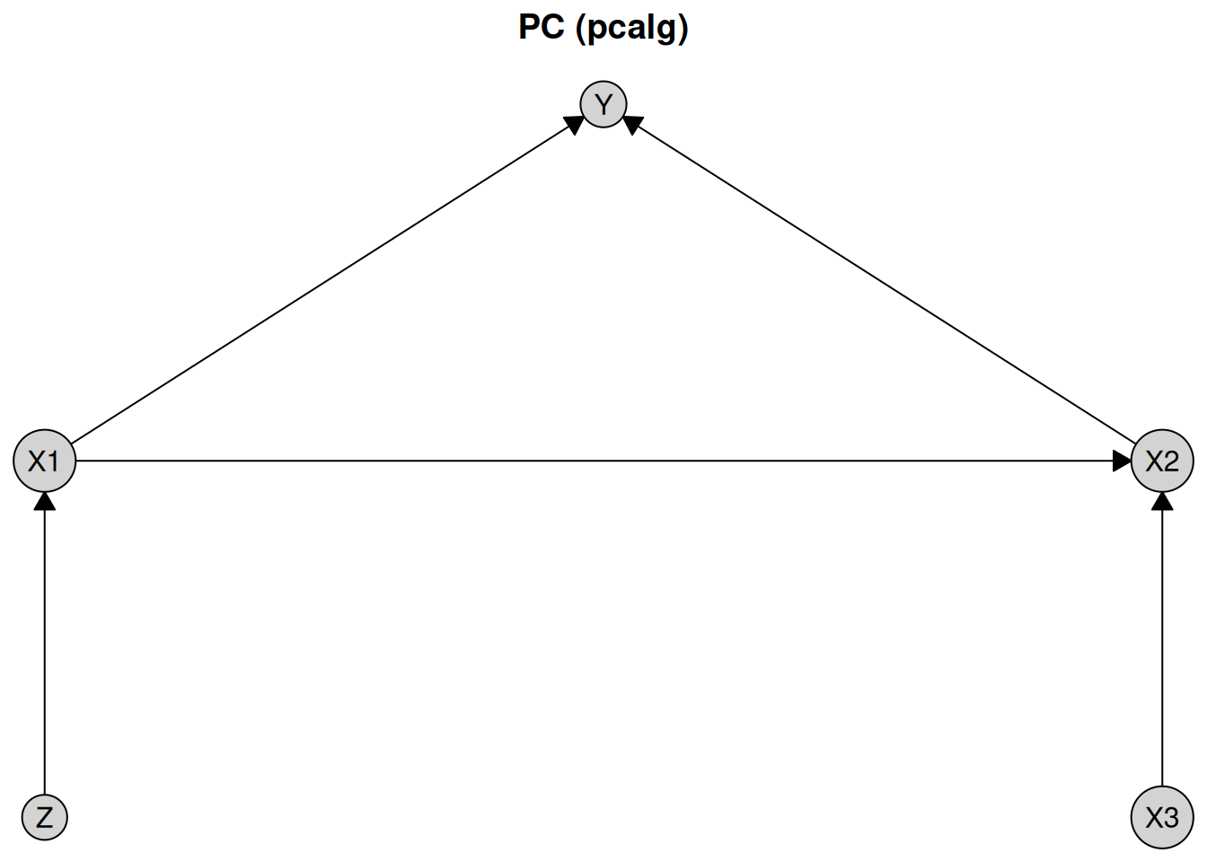
We see that the PC algorithm does not recover the correct causal structure due to the presence of the unobserved confounder. In particular, it found an incorrect edge between X1 and X2.
Next steps
For more information about how to incorporate knowledge into causal discovery methods, see the knowledge article.
For more information about how to visualize causal discovery results, see the visualization article.