library(causalDisco)
#> causalDisco startup:
#>   Java heap size requested: 2 GB
#>   Tetrad version: 7.6.10
#>   Java successfully initialized with 2 GB.
#>   To change heap size, set options(java.heap.size = 'Ng') or Sys.setenv(JAVA_HEAP_SIZE = 'Ng') *before* loading.
#>   Restart R to apply changes.
This article demonstrates how to visualize causal graphs. We cover plotting Knowledge objects and Disco objects, customizing layouts and styles, and exporting graphs to readable TikZ for inclusion and further customization in LaTeX documents.
Plotting
You can visualize causal graphs using the plot() function, which works for both Knowledge and Disco objects. The function leverages the underlying caugi::plot() method, providing flexible options for customizing the appearance of nodes and edges.
Plotting Knowledge Objects
We will use the dataset num_data for the following examples, which contains 5 numeric variables (X1, X2, X3, Y, and Z). We start by creating a simple Knowledge object and visualizing it with plot().
data(num_data)
kn <- knowledge(
  num_data,
  X1 %-->% c(X2, X3), # Require edge from X1 to X2, and X1 to X3
  X2 %!-->% c(X3, Y), # Forbid edge from X2 to X3, and X2 to Y
  Y %!-->% Z # Forbid edge from Y to Z
)

plot(kn)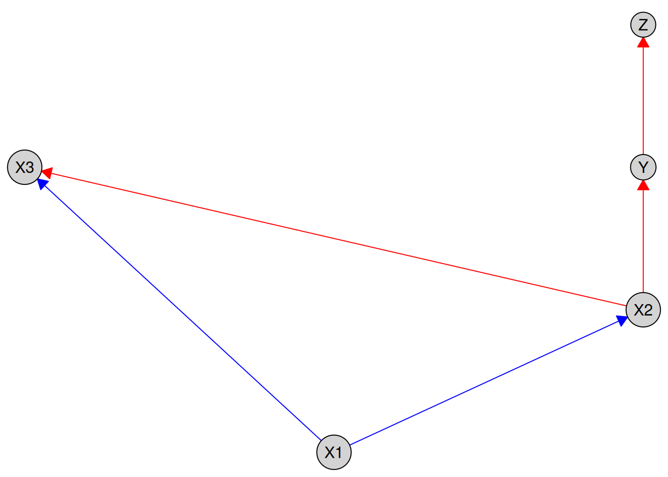
By default, required edges are shown in blue and forbidden edges in red. You can customize these colors using the required_col and forbidden_col arguments:
plot(kn, required_col = "skyblue", forbidden_col = "orange")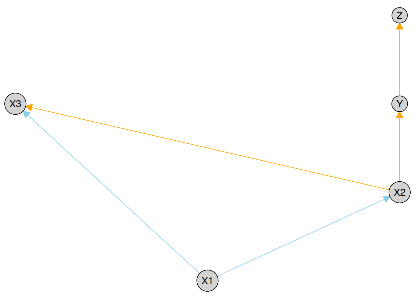
Different node layouts, node styles, and edge styles can be controlled via the layout, node_style, and edge_style parameters. We illustrate this with a simple example below. For a full description of available options, see the documentation for causalDisco::plot(), as well as the underlying caugi::plot() function and its visualization vignette (vignette("visualization", "caugi")).
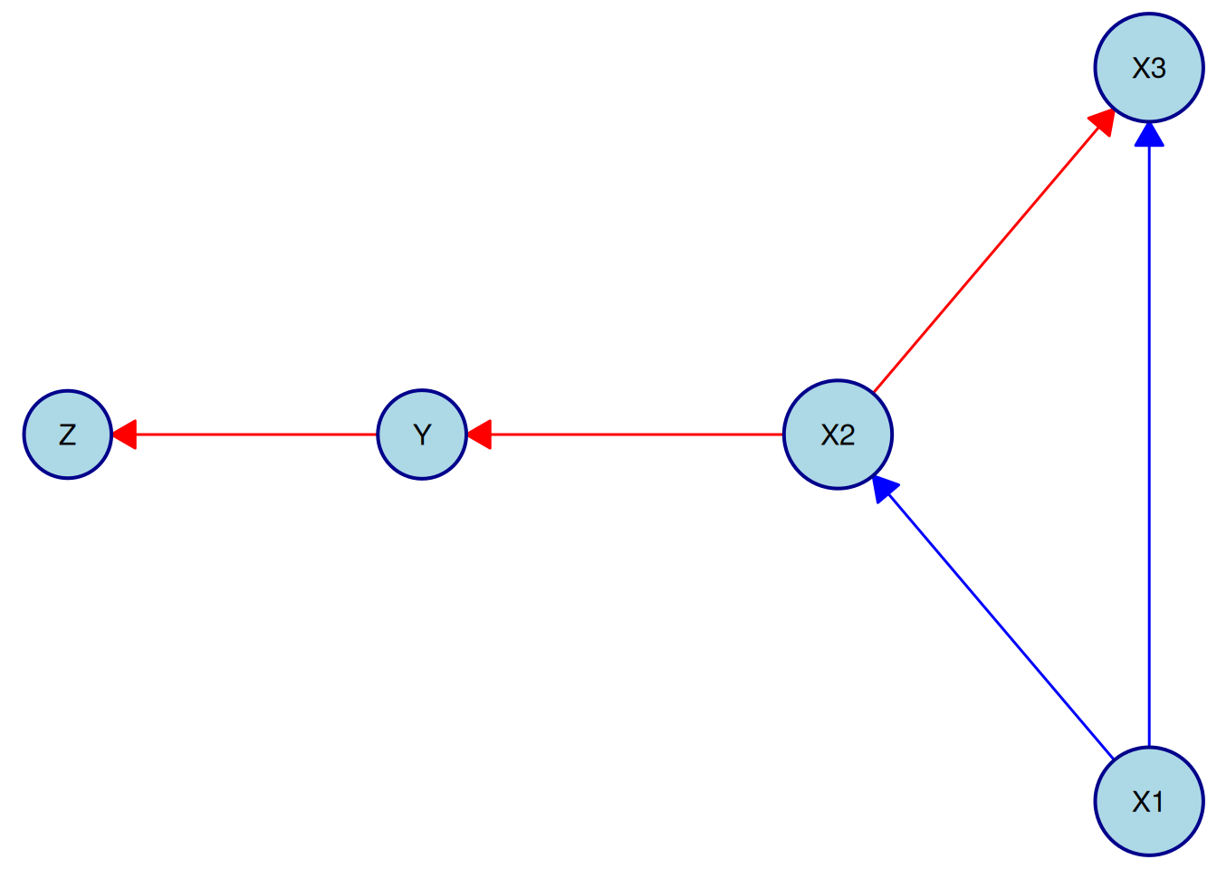
Here we use the "fruchterman-reingold" layout and customize node and edge styles:
plot(
  kn,
  layout = "fruchterman-reingold",
  node_style = list(
    fill = "lightblue", # Fill color
    col = "darkblue", # Border color
    lwd = 2, # Border width
    padding = 4, # Text padding (mm)
    size = 1.2 # Size multiplier
  ),
  edge_style = list(
    lwd = 1.5, # Edge width
    arrow_size = 4 # Arrow size (mm)
  ),
  required_col = "blue", # Color for required edges
  forbidden_col = "red" # Color for forbidden edges
)
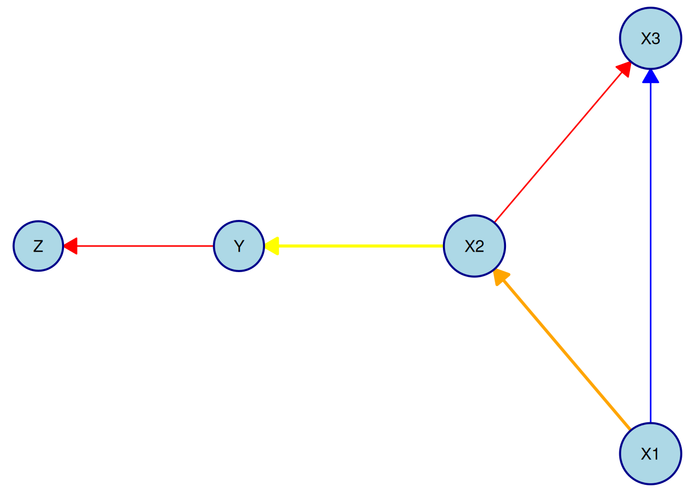
Note that to override the colors for required and forbidden edges only for a specific edge, the edge needs to be targeted explicitly in the by_edge list of the edge_style argument. For example, to make the required edge from X1 to X2 orange and the forbidden edge from X2 to Y yellow, while letting all other edges use the default colors, we can do:
plot(
  kn,
  layout = "fruchterman-reingold",
  node_style = list(
    fill = "lightblue", # Fill color
    col = "darkblue", # Border color
    lwd = 2, # Border width
    padding = 4, # Text padding (mm)
    size = 1.2 # Size multiplier
  ),
  edge_style = list(
    lwd = 1.5, # Edge width
    arrow_size = 4, # Arrow size (mm)
    # Per-edge overrides
    by_edge = list(
      X1 = list(
        X2 = list(col = "orange", fill = "orange", lwd = 3)
      ),
      X2 = list(
        Y = list(col = "yellow", fill = "yellow", lwd = 3)
      )
    )
  ),
  required_col = "blue", # Color for required edges
  forbidden_col = "red" # Color for forbidden edges
)
You can also pass a custom layout to plot():
my_layout <- data.frame(
  name = c("X1", "X2", "X3", "Y", "Z"),
  x = c(1, 2, 3, 4, 5),
  y = c(1, 2, 1, 2, 1)
)
plot(kn, layout = my_layout)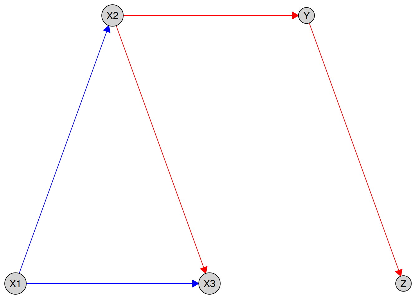
Plotting Tiered Knowledge
We can also visualize tiered knowledge structures. Here is an example using a dataset with variables measured at different life stages:
data(tpc_example)
kn_tiered <- knowledge(
  tpc_example,
  tier(
    child ~ starts_with("child"), # tidyselect helper; equivalent to c("child_x1", "child_x2")
    youth ~ starts_with("youth"),
    old ~ starts_with("old")
  ),
  child_x1 %-->% child_x2,
  child_x2 %!-->% youth_x3
)
plot(kn_tiered)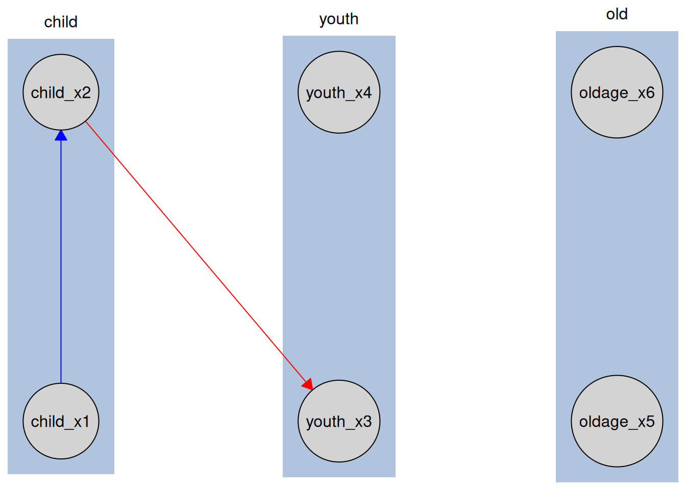
Variables are grouped by life stage, reflecting the tiered structure. This helps visually convey temporal or hierarchical relationships in the data.
Plotting Knowledgeable Caugi Objects
Here we run a causal discovery algorithm to get a Disco object, which is the knowledge object alongside the learned causal graph as a caugi::caugi object. We can then plot this combined object to see both the prior knowledge and the learned relationships
data(num_data)
kn <- knowledge(
  num_data,
  X1 %-->% X2,
  X2 %!-->% c(X3, Y),
  Y %!-->% Z
)

pc_bnlearn <- pc(engine = "bnlearn", test = "fisher_z")
pc_result <- disco(num_data, method = pc_bnlearn, knowledge = kn)
plot(pc_result)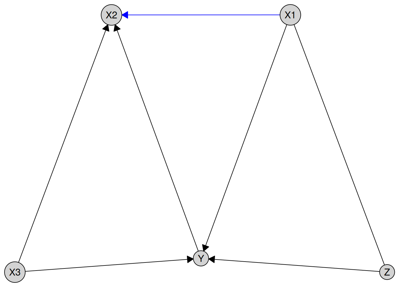
Blue edges indicate required relationships from prior knowledge, black edges show those learned from the data, and forbidden edges are not plotted (to avoid confusion and clutter).
With tiered knowledge, the plotting works similarly:
data(tpc_example)
kn_tiered <- knowledge(
  tpc_example,
  tier(
    child ~ starts_with("child"),
    youth ~ starts_with("youth"),
    old ~ starts_with("old")
  )
)
cd_tges <- tges(engine = "causalDisco", score = "tbic")
disco_cd_tges <- disco(
  data = tpc_example,
  method = cd_tges,
  knowledge = kn_tiered
)
plot(disco_cd_tges)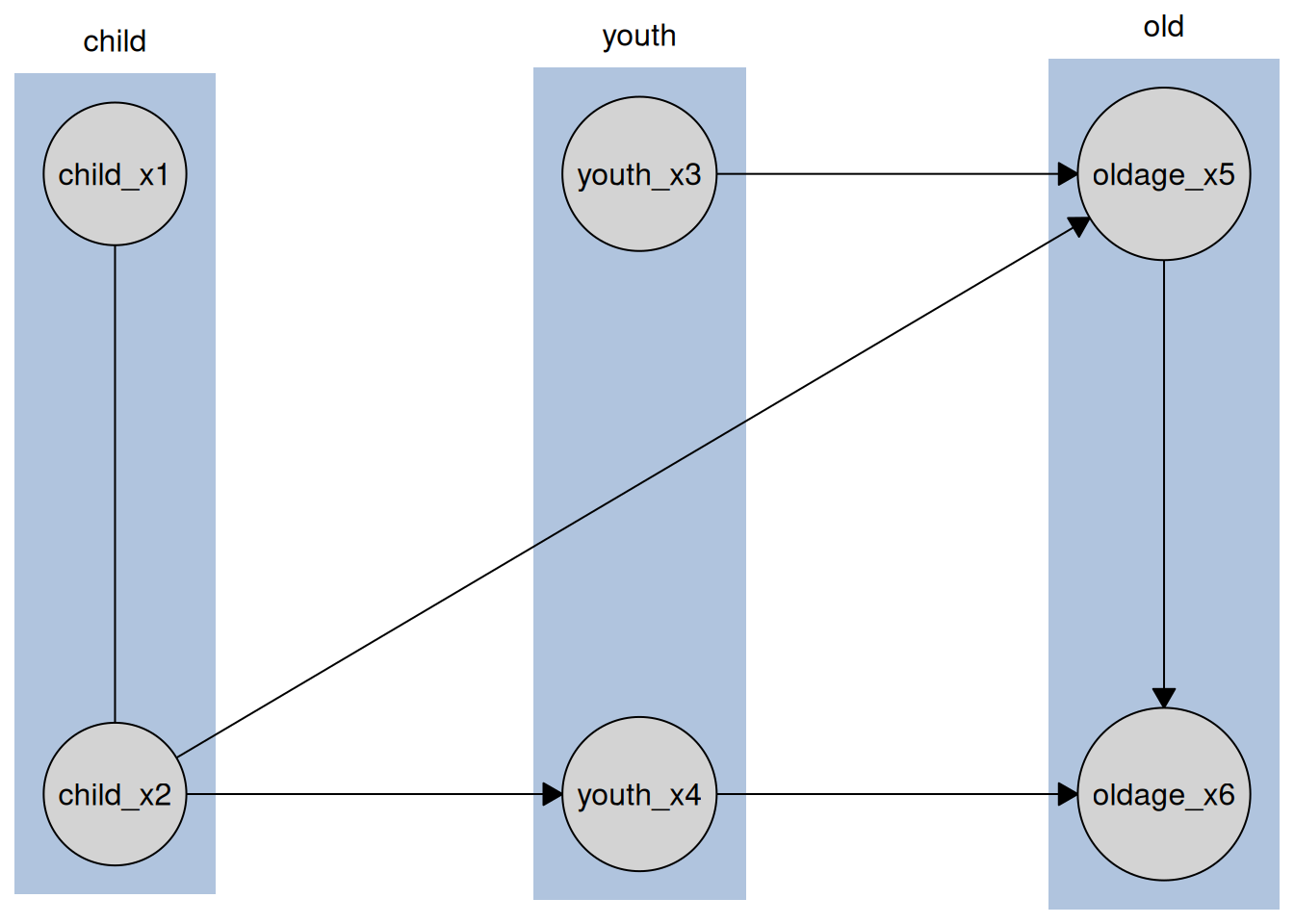
Where we can see the tiers reflected in the layout of the graph.
Exporting to TikZ
The make_tikz() function exports plots as clean, fully editable TikZ code for inclusion in LaTeX documents.
Unlike some graph export tools, edges are attached to nodes rather than positioned using hard-coded coordinates, making the output easier to modify.
This functionality works for Knowledge, Disco, and caugi::caugi objects, allowing you to customize layouts, styles, and edges further in your LaTeX document. It calls the underlying causalDisco::plot() method (which calls caugi::plot()) to generate the initial plot object before converting it to TikZ code. Thus, you can supply any arguments to make_tikz() that are supported by causalDisco::plot() and caugi::plot().
Exporting Knowledge to TikZ
We first demonstrate TikZ export for a Knowledge object.
data(num_data)
kn <- knowledge(
  num_data,
  X1 %-->% X2,
  X2 %!-->% c(X3, Y),
  Y %!-->% Z
)

# Full standalone document
tikz_knowledge_code <- make_tikz(kn, scale = 10, full_doc = TRUE)
cat(tikz_knowledge_code)
#> %%% Generated by causalDisco (version 1.1.0.9000)
#> \documentclass[tikz,border=2mm]{standalone}
#> \usetikzlibrary{arrows.meta, positioning, shapes.geometric, fit, backgrounds, calc}
#>
#> \begin{document}
#> \tikzset{every node/.style={fill=lightgray}, every path/.style={draw=red}}
#> \tikzset{arrows={[scale=3]}, arrow/.style={-{Stealth}, thick}}
#> \begin{tikzpicture}
#> \node[draw, circle] (X1) at (1.667,0) {X1};
#> \node[draw, circle] (X2) at (1.667,3.333) {X2};
#> \node[draw, circle] (X3) at (3.333,6.667) {X3};
#> \node[draw, circle] (Y) at (0,6.667) {Y};
#> \node[draw, circle] (Z) at (0,10) {Z};
#> \path (X1) edge[draw=blue, -Latex] (X2)
#>       (X2) edge[, -Latex] (X3)
#>       (X2) edge[, -Latex] (Y)
#>       (Y) edge[, -Latex] (Z);
#> \end{tikzpicture}
#> \end{document}

# Only the tikzpicture environment
tikz_knowledge_snippet <- make_tikz(kn, scale = 10, full_doc = FALSE)
cat(tikz_knowledge_snippet)
#> %%% Generated by causalDisco (version 1.1.0.9000)
#> \tikzset{every node/.style={fill=lightgray}, every path/.style={draw=red}}
#> \tikzset{arrows={[scale=3]}, arrow/.style={-{Stealth}, thick}}
#> \begin{tikzpicture}
#> \node[draw, circle] (X1) at (1.667,0) {X1};
#> \node[draw, circle] (X2) at (1.667,3.333) {X2};
#> \node[draw, circle] (X3) at (3.333,6.667) {X3};
#> \node[draw, circle] (Y) at (0,6.667) {Y};
#> \node[draw, circle] (Z) at (0,10) {Z};
#> \path (X1) edge[draw=blue, -Latex] (X2)
#>       (X2) edge[, -Latex] (X3)
#>       (X2) edge[, -Latex] (Y)
#>       (Y) edge[, -Latex] (Z);
#> \end{tikzpicture}
Setting full_doc = TRUE generates a complete standalone LaTeX document that can be compiled directly. Using full_doc = FALSE instead returns only the tikzpicture environment, which is convenient for inclusion inside an existing LaTeX document.
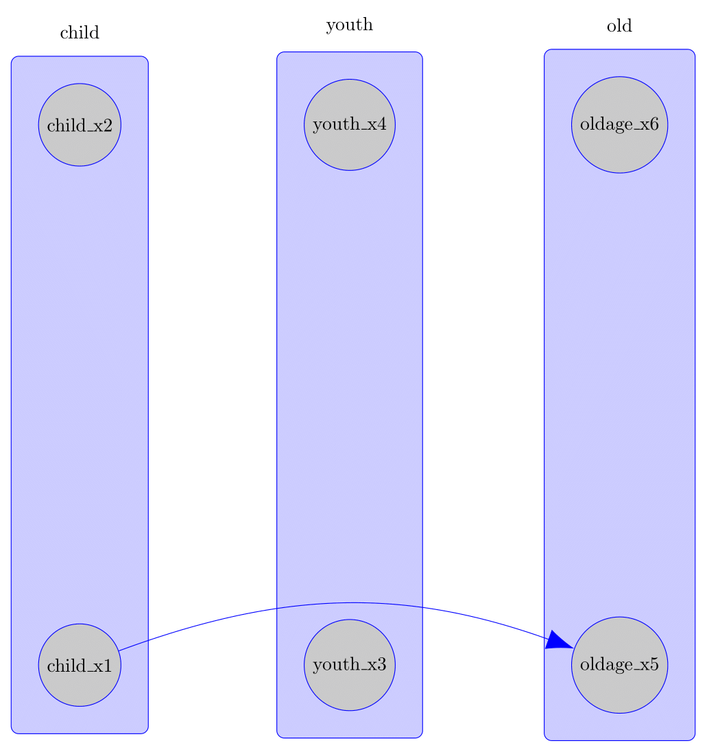
The TikZ export also supports edge bending, which can substantially improve readability when edges pass through other nodes, as can easily happen in tiered knowledge structures. This feature is not available in the standard caugi::plot() function. Here is an example, where the edge using the standard straight style edge overlaps the node youth_x3, while the bent edge avoids this overlap:
data(tpc_example)
kn_tiered <- knowledge(
  tpc_example,
  tier(
    child ~ starts_with("child"),
    youth ~ starts_with("youth"),
    old ~ starts_with("old")
  ),
  child_x1 %-->% oldage_x5
)

plot(kn_tiered)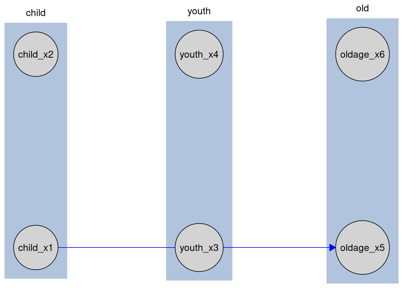
tikz_bent_tiered <- make_tikz(
  kn_tiered,
  scale = 10,
  full_doc = FALSE,
  bend_edges = TRUE,
  bend_angle = 20
)
cat(tikz_bent_tiered)
#> %%% Generated by causalDisco (version 1.1.0.9000)
#> \tikzset{every node/.style={fill=lightgray}, every path/.style={draw=blue}}
#> \tikzset{arrows={[scale=3]}, arrow/.style={-{Stealth}, thick}}
#> \begin{tikzpicture}
#> \node[draw, circle] (child_x1) at (0,0) {child\_x1};
#> \node[draw, circle] (child_x2) at (0,10) {child\_x2};
#> \node[draw, circle] (youth_x3) at (5,0) {youth\_x3};
#> \node[draw, circle] (youth_x4) at (5,10) {youth\_x4};
#> \node[draw, circle] (oldage_x5) at (10,0) {oldage\_x5};
#> \node[draw, circle] (oldage_x6) at (10,10) {oldage\_x6};
#> \begin{scope}[on background layer]
#> \node[draw, rectangle, fill=blue!20, rounded corners, inner sep=0.5cm, fit=(child_x1)(child_x2)] (child) {};
#> \node[draw, rectangle, fill=blue!20, rounded corners, inner sep=0.5cm, fit=(oldage_x5)(oldage_x6)] (old) {};
#> \node[draw, rectangle, fill=blue!20, rounded corners, inner sep=0.5cm, fit=(youth_x3)(youth_x4)] (youth) {};
#> \end{scope}
#> \node[anchor=south, draw=none, fill=none] at ($(child.north)+(0cm,0.2cm)$) {child};
#> \node[anchor=south, draw=none, fill=none] at ($(old.north)+(0cm,0.2cm)$) {old};
#> \node[anchor=south, draw=none, fill=none] at ($(youth.north)+(0cm,0.2cm)$) {youth};
#> \path (child_x1) edge[bend left=20, -Latex] (oldage_x5);
#> \end{tikzpicture}
The TikZ plot can be seen here:
Exporting Knowledgeable Caugi to TikZ
The output of disco() gives a Disco object, which can also be exported to TikZ:
data(tpc_example)
kn_tiered <- knowledge(
  tpc_example,
  tier(
    child ~ starts_with("child"),
    youth ~ starts_with("youth"),
    old ~ starts_with("old")
  )
)

cd_tges <- tges(engine = "causalDisco", score = "tbic")
disco_cd_tges <- disco(
  data = tpc_example,
  method = cd_tges,
  knowledge = kn_tiered
)

tikz_snippet <- make_tikz(
  disco_cd_tges,
  scale = 10,
  full_doc = FALSE
)
cat(tikz_snippet)
#> %%% Generated by causalDisco (version 1.1.0.9000)
#> \tikzset{every node/.style={fill=lightgray}}
#> \tikzset{arrows={[scale=3]}, arrow/.style={-{Stealth}, thick}}
#> \begin{tikzpicture}
#> \node[draw, circle] (child_x2) at (0,0) {child\_x2};
#> \node[draw, circle] (child_x1) at (0,10) {child\_x1};
#> \node[draw, circle] (youth_x4) at (5,0) {youth\_x4};
#> \node[draw, circle] (youth_x3) at (5,10) {youth\_x3};
#> \node[draw, circle] (oldage_x6) at (10,0) {oldage\_x6};
#> \node[draw, circle] (oldage_x5) at (10,10) {oldage\_x5};
#> \begin{scope}[on background layer]
#> \node[draw, rectangle, fill=blue!20, rounded corners, inner sep=0.5cm, fit=(child_x1)(child_x2)] (child) {};
#> \node[draw, rectangle, fill=blue!20, rounded corners, inner sep=0.5cm, fit=(oldage_x5)(oldage_x6)] (old) {};
#> \node[draw, rectangle, fill=blue!20, rounded corners, inner sep=0.5cm, fit=(youth_x3)(youth_x4)] (youth) {};
#> \end{scope}
#> \node[anchor=south, draw=none, fill=none] at ($(child.north)+(0cm,0.2cm)$) {child};
#> \node[anchor=south, draw=none, fill=none] at ($(old.north)+(0cm,0.2cm)$) {old};
#> \node[anchor=south, draw=none, fill=none] at ($(youth.north)+(0cm,0.2cm)$) {youth};
#> \path (child_x1) edge[, -] (child_x2)
#>       (child_x2) edge[, -Latex] (oldage_x5)
#>       (child_x2) edge[, -Latex] (youth_x4)
#>       (oldage_x5) edge[, -Latex] (oldage_x6)
#>       (youth_x3) edge[, -Latex] (oldage_x5)
#>       (youth_x4) edge[, -Latex] (oldage_x6);
#> \end{tikzpicture}
Exporting Caugi Objects to TikZ
The same export mechanism also applies to standard caugi::caugi objects:
cg <- caugi::caugi(
  A %-->% B + C
)
plot_obj <- caugi::plot(cg, node_style = list(fill = "red"))
tikz_caugi_snippet <- make_tikz(plot_obj, scale = 10, full_doc = FALSE)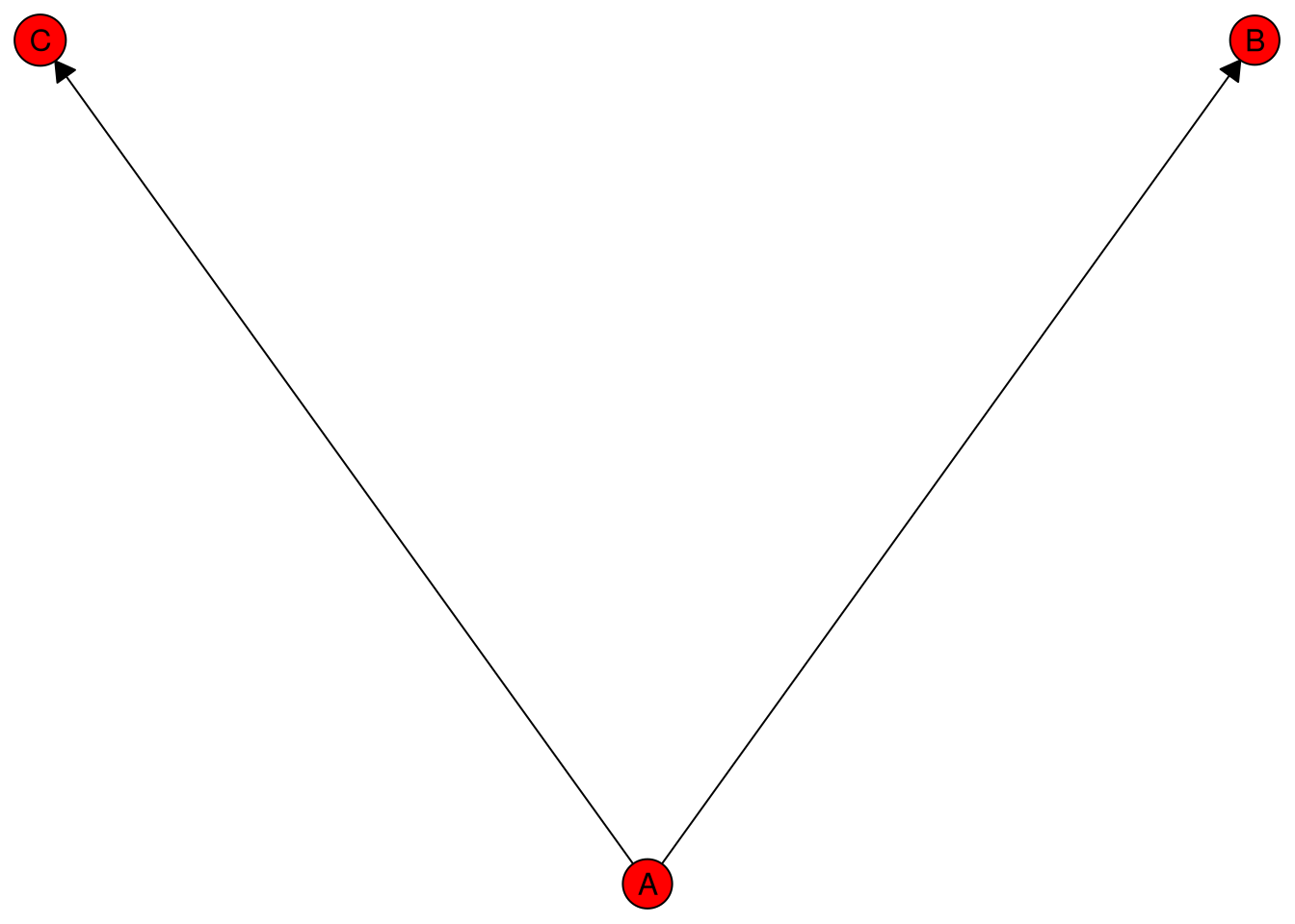
cat(tikz_caugi_snippet)
#> %%% Generated by causalDisco (version 1.1.0.9000)
#> \tikzset{every node/.style={fill=red}}
#> \tikzset{arrows={[scale=3]}, arrow/.style={-{Stealth}, thick}}
#> \begin{tikzpicture}
#> \node[draw, circle] (A) at (5,0) {A};
#> \node[draw, circle] (B) at (10,10) {B};
#> \node[draw, circle] (C) at (0,10) {C};
#> \path (A) edge[, -Latex] (B)
#>       (A) edge[, -Latex] (C);
#> \end{tikzpicture}